Matt's Matlab Tutorial Source Code Page
This document contains a tutorial on
Matlab
with a principal components analysis for a set of face images as the
theme.
I wrote this tutorial while a graduate student in the
Artificial Intelligence Laboratory of
the Computer Science and Engineering
Department at the University of California,
San Diego. Now it's here at
CSIM-AIT.
You might still be able to find the original
here.
 This work is licensed under a
Creative
Commons Attribution 3.0 License. You are free to use the code here for
any purpose you like, but please acknowledge its source if you do. It's not
required, but if you make improvements I'd appreciate it if you sent me your
updates.
Here's an index to this tutorial:
I used the Ekman and Friesen Pictures of Facial Affect (POFA) for this
tutorial. Unfortunately, the faces are copyrighted so if you want them
you'll have to pay Paul Ekman some cash to get our online version of
the database. Contact Gary Cottrell
for details about our versions, or see
http://www.paulekman.com/researchproducts.html
on getting a CD directly from Ekman.
Don't despair, however. There are a bunch of nice face databases that
are free. Check the
Face Recognition
Home Page for a list of what's available.
What is PCA and the “Eigenface”
Technique?
I won't go into it in detail here, but the idea is that face images
can be economically represented by their projection onto a small number
of basis images that are derived by finding the most significant
eigenvectors of the pixelwise covariance matrix for a set of training
images.
A quick
Google
Search shows that a lot of people like to play with this technique.
In my tutorial I simply show how to get some eigenfaces and play with them
in Matlab.
If you don't use emacs, the Matlab emacs mode may be one reason to use it.
To get Matlab mode working in emacs, put matlab.el
somewhere emacs can find it and add something like the following to your
.emacs file:
(autoload 'matlab-mode "matlab" "Enter Matlab mode." t)
(setq auto-mode-alist (cons '("\\.m$" . matlab-mode) auto-mode-alist))
(defun my-matlab-mode-hook ()
  (setq matlab-indent-function t)       ; if you want function bodies indented
  (setq fill-column 76)         ; where auto-fill should wrap
  (matlab-mode-hilit)
  (turn-on-auto-fill))
(setq matlab-mode-hook 'my-matlab-mode-hook)
(autoload 'matlab-shell "matlab" "Interactive Matlab mode." t)
(defun my-matlab-shell-mode-hook ()
  '())
(setq matlab-mode-hook 'my-matlab-mode-hook)
I don't pretend to understand any of this emacs stuff. For more information,
you might try the
Mathworks Matlab Central Contrib site.
Matlab can read PNG files and other formats without help. Here is how
to read a PNG image into memory and look at the pixel values in its upper
left corner. The ">>" is the Matlab prompt. Comments begin with a
% sign.
>> help imread                    % Online help is useful...

 IMREAD Read image from graphics file.
    A = IMREAD(FILENAME,FMT) reads the image in FILENAME into
    A. If the file contains a grayscale intensity image, A is
    a two-dimensional array.  If the file contains a truecolor

    etc...

>> I = imread('test.png');        % Read image test.png into variable I
>> size(I)                        % Get the number of rows and columns of I

ans =

   320   240

>> I(1:10,1:10)                   % Display row 1-10 and col 1-10 of I

ans =

    26    20    20    22    22    20    19    20    22    22
    26    24    19    22    22    19    21    24    24    22
    25    24    22    24    21    19    20    22    24    22
    25    21    21    24    22    20    21    22    24    20
    24    20    22    25    22    19    20    21    25    24
    20    19    22    22    24    21    21    24    22    24
    20    20    21    25    25    24    24    25    20    20
    20    20    21    24    26    25    25    25    20    20
    20    19    22    24    24    25    24    24    22    21
    21    17    21    25    21    22    24    25    22    21

>> colormap(gray(256));          % Use a 256-value grayscale color map
>> image(I);                     % Display I as an image
>> daspect([1 1 1]);             % Set x:y aspect ratio to be 1:1
If you like the PGM format like I do, here are matlab functions for reading
and writing them:
Matlab is really nice for linear algebra stuff and visualization, but sorta
sucks when it comes to file I/O. Or rather, it's not much easier than C,
although there are functions for reading and writing entire arrays to and
from files. The following function, defined in
load_images.m, is an example of how to read
a bunch of images, make column vectors out of each of them, and return the
result.
function [Images,w,h] = load_images(filelist,downscale_f)
%LOAD_IMAGES Load a set of images listed in a file.
%
%            [IMGS,W,H] = LOAD_IMAGES(FILELIST) Treat each line of
%            the file named FILELIST as the filename of a PGM image,
%            and load each image as one column of the return array
%            IMGS.
%
%            LOAD_IMAGES(FILELIST,DOWNSCALE_F) Do the same thing,
%            but downscale each image's width and height by a factor
%            of DOWNSCALE_F.  Useful if the images are too big to be
%            loaded into memory all at once.

% Matthew Dailey 2000

  % Check argument consistency

  if nargin < 1 | nargin > 2
    error('usage: load_images(filelist[,downscale_f]');
  end;
  if nargin == 1
    downscale_f = 1.0;
  end;
  Images = []; old_w = 0; old_h = 0; w=0; h=0;

  % Open input file

  numimgs = linecount(filelist);
  fid = fopen(filelist,'r');
  if fid < 0 | numimgs < 1
    error(['Cannot get list of images from file "' filelist, '"']);
  end;

  % Get the images

  for i = 1:numimgs
    imgname = fgetl(fid);
    if ~isstr(imgname)            % EOF is not a string
      break;                      % Exit from loop on EOF
    end;
    fprintf(1,'loading PGM file %s\n',imgname);
    Img = readpgm(imgname);       % Read this image as a 2D array
    if i==1                       % If this is first image, figure things out
      old_w = size(Img,2);        %   - like sizes of the downscaled images
      old_h = size(Img,1);
      if downscale_f <= 1.0
	w = old_w; h = old_h;
      else
	w = round(old_w/downscale_f); h = round(old_h/downscale_f);
      end;
      Images = zeros(w*h,numimgs);   % - preallocate size of the return matrix
    end;
    if downscale_f > 1.0
      Img = im_resize(Img,w,h);      % downscale using bicubic spline interp
    end;
    Images(1:w*h,i) = reshape(Img',w*h,1);   % Make a column vector
  end;
  fclose(fid);                    % Close the filelist when done

  fprintf(1,'Read %d images.\n',numimgs);

  % The function returns the output arguments Images, w, and h here.
The function has a downscaling factor that lets you save memory.
To use the function, just create a file listing your images then run:
>> [Imgs,w,h] = load_images('facelist',4);
The im_resize function uses Matlab's built in
2-D function interpolation (using bicubic splines) to resize the image
by the desired downscaling factor. If you want to run load_images,
you also need the trivial little function linecount.
Here is how you would convert a column of Imgs back into an image
and display it:
>> L = Imgs(:,10);
>> L = reshape(L,w,h)';         % Reshapes column vector into a 2D array
>> image(L);
>> colormap(gray(256));
>> daspect([1 1 1]);
The function pc_evectors uses Turk and Pentland's
trick to get the eigenvectors of A*A' from the eigenvectors of A'*A.
It uses the function sortem to sort the eigenvectors
and eigenvalues by eigenvalue. [Here is a faster version,
sortem2, by James
Javurek-Humig,
which is considerably faster, if you have matlab version 7 or better.]
To use pc_evectors, just do:
>> [Vecs,Vals,Psi] = pc_evectors(Imgs,30); % Get top 30 PC evectors of Imgs
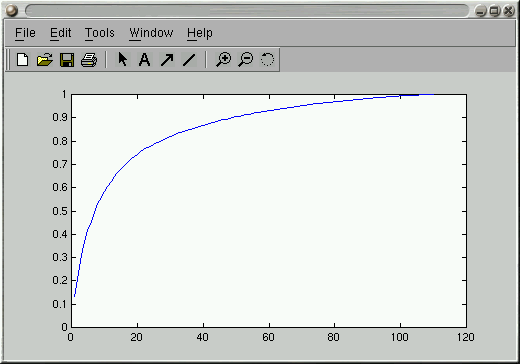
And to explore the eigenvalue spectrum and how much variance the first
n vectors account for, try the following:
>> plot(Vals);                       % To plot the eigenvalues
>> CVals = zeros(1,length(Vals));    % Allocate a vector same length as Vals
>> CVals(1) = Vals(1);
>> for i = 2:length(Vals)            % Accumulate the eigenvalue sum
     CVals(i) = CVals(i-1) + Vals(i);
   end;
>> CVals = CVals / sum(Vals);        % Normalize total sum to 1.0
>> plot(CVals);                      % Plot the cumulative sum
>> ylim([0 1]);                      % Set Y-axis limits to be 0-1
This gives you something like the following:

It depends on the application, but most folks seem to use a number of
eigenvectors that account for variance somewhere in the 65%-90% range.
One thing that can be fun is to try to figure out what the top few
eigenvectors encode. You can make a scatter plot of one component
against another as follows:
>> Proj = Vecs(:,1:2)' * Imgs;       % Project each image onto first 2 evectors
>> size(Proj)

ans =

     2   110

>> plot(Proj(1,:),Proj(2,:),'r.')    % To get scatterplot of PC 1 vs PC 2
And if you wanted to add text labels to each of the points in the plot,
you could do the following. First create a file containing the labels
you want, in the correct order. Then read it into a Matlab string array:
>> Labels = textread('labels','%s');    % Read labels from file 'labels'
>> text(Proj(1,:),Proj(2,:),Labels);    % Add text labels at each plotted point
It is simple to display an eigenface as an image, using the
built in imagesc function, which first scales the values in an array
to the 0-255 range.
>> pc_ev_1 = Vecs(:,1);                 % Get PC eigenvector 1
>> pc_ev_1 = reshape(pc_ev_1,w,h)';     % Reshape into 2D array
>> imagesc(pc_ev_1);                    % Display as image scaled 0-255
Finally, you might be interested in determining the reconstruction
error involved in representing an image by its projection onto a few
eigenvectors. Here is how you would project onto and reconstruct from
eigenvectors 1-10.
>> OrigImg = Imgs(:,20);                     % Grab image 20
>> Projection = Vecs(:,1:10)'*(OrigImg - Psi);    % Project onto ev's 1-10
>> Reconstruction = Vecs(:,1:10)*Projection+Psi;  % Reconstruct from projection
>> Reconstruction = reshape(Reconstruction,w,h)';
>> image(Reconstruction);
>> colormap(gray(256));
>> daspect([1 1 1]);
- Turk, M. and Pentland, A. (1991). Eigenfaces for recognition.
The Journal of Cognitive Neuroscience, 3(1): 71-86.
- The photo of Kurt Cobain, representing the fact that this tutorial
was written on a Linux box named after him, originally came from
http://mrshowbiz.go.com/people/kurtcobain/content/bio.html
but the original site is long gone. Now the original
photographer is unknown.
mdailey@ait.ac.th
http://www.cs.ait.ac.th/~mdailey
 This work is licensed under a
Creative
Commons Attribution 3.0 License. You are free to use the code here for
any purpose you like, but please acknowledge its source if you do. It's not
required, but if you make improvements I'd appreciate it if you sent me your
updates.

